UnMix-TNS

Summary

We introduce a novel test-time normalization scheme (UnMix-TNS) designed to withstand the challenges posed by label temporal correlation of test data streams.
UnMix-TNS demonstrates robustness across various test-time distribution shifts such as single domain, and continual domain. While not primarily designed for mixed domain settings, it offers a level of adaptability in these scenarios. Additionally, the method excels with small batch sizes, even down to individual samples.
UnMix-TNS layers, with negligible inference latency, seamlessly integrate into pre-trained neural network architectures, fortified with BN layers, augmenting test-time adaptation strategies while incurring minimal overhead.
We present empirical evidence showcasing significant performance improvements of state-of-the-art TTA methods in non-i.i.d. settings when augmented with UnMix-TNS, as benchmarked on datasets involving common corruptions shifts and natural shifts.

Motivation

To elucidate the motivation of our method, let's compare it with the conventional approach of test-time batch normalization (TBN), using a toy example for clarity.

I.I.D Setting. Under i.i.d setting, the feature statistics estimated from the current batch (pink dots) is close to the true statistics of the test distribution.
Non-I.I.D Setting. Under non-i.i.d. setting (i.e. when the test features are label temporally correlated), the feature statistics estimated from the current batch are biased towards one category.
Our Method. To address this imbalance issue, we introduce a novel strategy termed UnMix-TNS (Un-Mixing Test-Time Normalization Statistics) simulating the i.i.d. setting by splitting the statistics of the test distribution into K components (4 in this example), and estimating them using only the test features closest to the individual component.

Figure: Illustration comparing UnMix-TNS with the TBN approach using a toy example in i.i.d. and non-i.i.d. settings.

Method: UnMix-TNS

1. Distribution of \(K\) UnMix-TNS Components Mixture

Task Affinity Diagram — **Figure:** **An Overview of UnMix-TNS.** Given a batch of non-i.i.d test features \( \mathbf{z^t} \in \mathbb{R}^{B \times C \times L} \) at a temporal instance \( t \), we mix the instance-wise statistics \( (\tilde{\mu}^t, \tilde{\sigma}^t) \in \mathbb{R}^{B \times C} \) with \( K \) UnMix-TNS components. The alignment of each sample in the batch with the UnMix-TNS components is quantified through similarity-derived assignment probabilities \( p_k^t \). This aids both the *mixing* process and subsequent component updates for time \( t+1 \).

Let \( [\mu_1^t, \dots, \mu_K^t] \) and \( [\sigma_1^t, \dots, \sigma_K^t] \) denote the statistics of the \( K \) components within the UnMix-TNS layer at a given temporal instance \( t \), where each \( \mu_k^t, \sigma_k^t \in \mathbb{R}^C \). We articulate the distribution \( h_Z^t(z) \) of instance-wise test features \( z \in \mathbb{R}^C \) marginalized over all labels at a temporal instance \( t \) using the \( K \) components:

\[ h_{Z_c}^t(z_c) = \frac{1}{K}\sum_k \mathcal{N}(\mu_{k,c}^t, \sigma_{k,c}^t), \]

where \( \mathcal{N} \) represents the Normal distribution function. Given only \( (\mu_k^t, \sigma_k^t)_{k=1}^{K} \), one can derive the label unbiased normalization test statistics \( (\bar{\mu}^t, \bar{\sigma}^t) \) at time \( t \) as follows:

\[ \bar{\mu}^t = \mathbb{E}_{h_{Z_c}^t}[z_c]=\frac{1}{K}\sum_k \mu_{k,c}^t, \]

\[ (\bar{\sigma}^t)^2 = \mathbb{E}_{h_{Z_c}^t}[(z_c-\bar{\mu}^t)^2]=\frac{1}{K}\sum_k (\sigma_{k,c}^t)^2 + \frac{1}{K}\sum_k (\mu_{k,c}^t)^2 - \Big(\frac{1}{K}\sum_k\mu_{k,c}^t\Big)^2, \]

Subsequent sections will delve into the initialization scheme for the \( K \) UnMix-TNS components and elucidate the process of updating their individual statistics \( (\mu_k^t, \sigma_k^t) \) at temporal instance \( t \).

2. Initializing UnMix-TNS Components

Consider the pair \( (\mu,\sigma) \in \mathbb{R}^C \), which stands as the stored means and standard deviation of the features in a given BN layer of \( f_\theta \), derived from the source training dataset before adaptation.

We initialize statistics \( (\mu_k^t, \sigma_k^t) \) of \( K \) components of UnMix-TNS at \( t=0 \), as delineated in the following Equation:

\[ \mu_{k,c}^0 = \mu_c + \sigma_c \sqrt{\frac{\alpha \cdot K}{K-1}} \cdot \zeta_{k,c}, \quad \sigma_{k,c}^0 = \sqrt{1-\alpha}\cdot\sigma_c, \quad \zeta_{k,c} \sim \mathcal{N}(0, 1) \]

where \( \zeta_{k,c} \) is sampled from the standard normal distribution \( \mathcal{N}(0, 1) \), and \( \alpha \in (0, 1) \) is a hyperparameter that controls the extent to which the means of the UnMix-TNS components deviate from the stored means of BN layer during initialization. Note that the initial normalization statistics \( (\bar{\mu}^0, \bar{\sigma}^0) \) estimated from \( (\mu_k^0, \sigma_k^0) \) have an expected value equal to the stored statistics of the BN layer, i.e., \( \mathbb{E}[\bar{\mu}^0_k]=\mu \) and \( \mathbb{E}[(\bar{\sigma}^0_k)^2] = \sigma^2 \) for all values of \( \alpha \).

3. Redefining Feature Normalization through UnMix-TNS

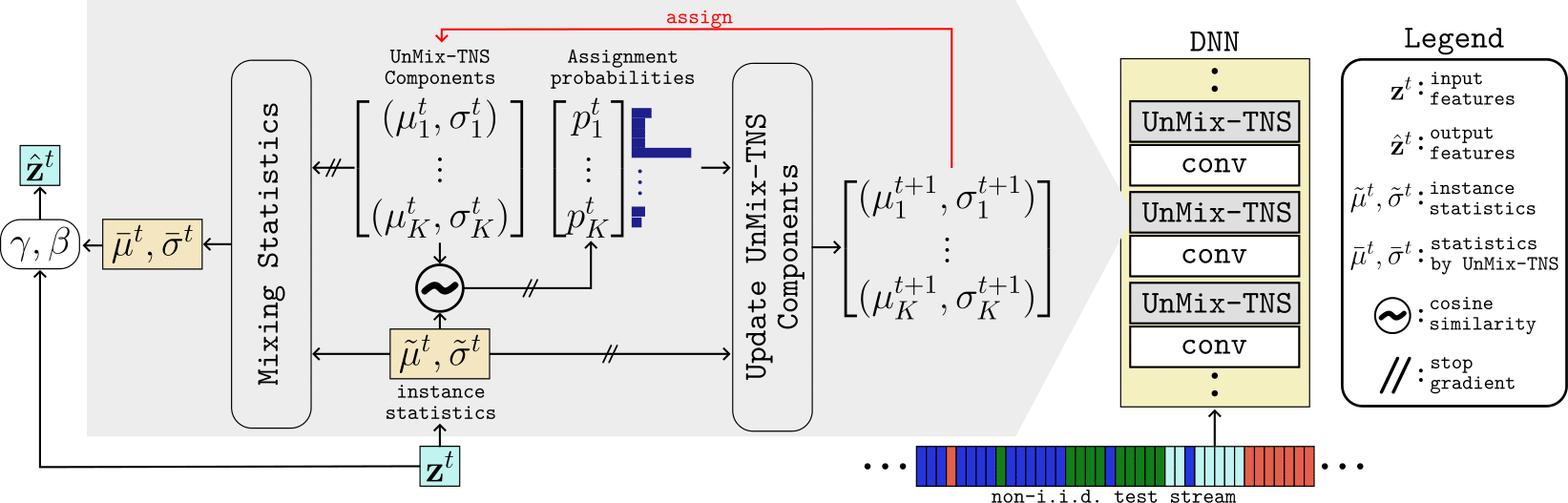
Considering the current batch of temporally correlated features \( \mathbf{z}^t \in \mathbb{R}^{B \times C \times L} \), we commence by calculating the instance-wise means and standard deviation \( (\tilde{\mu}^t, \tilde{\sigma}^t) \in \mathbb{R}^{B \times C} \), mirroring the Instance Normalization, i.e.:

\[ \tilde{\mu}^t_{b,c} = \frac{1}{L}\sum_{l} \mathbf{z}^t_{b,c,l},\quad \tilde{\sigma}^t_{b,c} =\sqrt{\frac{1}{L} \sum_l(\mathbf{z}^t_{b,c,l} - \tilde{\mu}^t_{b,c})^2}, \]

To gauge the likeness between UnMix-TNS components and current test features, we compute the cosine similarity \( s^t_{b,k} \) of the current instance-wise means \( \tilde{\mu}^t_{b,:} \) with that of \( K \) BN components \( \left \{ \mu_k^t \right \}_{k=1}^{K} \) as follows:

\[ s_{b,k}^t = \texttt{sim}\left ( \tilde{\mu}^t_{b,:},\mu_k^t \right ), \]

where \( \texttt{sim}(\mathbf{u},\mathbf{v})=\frac{\mathbf{u}^T\mathbf{v}}{\|\mathbf{u}\|\|\mathbf{v}\|} \) denote the dot product between \( l_2 \) normalized \( \mathbf{u} \) and \( \mathbf{v} \in \mathbb{R}^C \).

We proceed to derive the refined feature statistics, denoted as \( (\bar{\mu}^t, \bar{\sigma}^t) \in \mathbb{R}^{B \times C} \) for each instance. This is accomplished by a weighted mixing of the current instance statistics, \( (\tilde{\mu}^t, \tilde{\sigma}^t) \), harmoniously blended with the \( K \) BN statistics components, \( (\mu_k^t, \sigma_k^t)_{k=1}^K \). This mixing strategy unfolds similar to as:

\[ \bar{\mu}^t_{b,c} = \frac{1}{K}\sum_{k}\hat{\mu}^t_{b,k,c}, \]

\[ (\bar{\sigma}^t_{b,c})^2 = \frac{1}{K}\sum_{k}(\hat{\sigma}^t_{b,k,c})^2 + \frac{1}{K}\sum_{k}(\hat{\mu}^t_{b,k,c})^2 - \left(\frac{1}{K}\sum_k \hat{\mu}^t_{b,k,c}\right)^2, \]

\[ \hat{\mu}^t_{b,k,c} = (1-p_{b,k}^t) \cdot \mu_{k,c}^t + p_{b,k}^t \cdot \tilde{\mu}^t_{b,c}, \quad (\hat{\sigma}^t_{b,k,c})^2 = (1-p_{b,k}^t) \cdot (\sigma_{k,c}^t)^2 + p_{b,k}^t \cdot (\tilde{\sigma}^t_{b,c})^2, \]

In this formulation, \( p_{b,k}^t = \frac{\exp(s^t_{b,k}/\tau)}{\sum_\kappa \exp(s^t_{b,k}/\tau)} \) represents the assignment probability of the \( b^{th} \) instance's statistics in the batch belonging to the \( k^{th} \) statistics component. Note that, \( p_{b,k}^t\approx 1 \) if \( b^{th} \) instance exhibits a greater affinity to the \( k^{th} \) component, and vice-versa. We employ the refined feature statistics \( (\bar{\mu}^t, \bar{\sigma}^t) \) to normalize \( \mathbf{z}^t \), yielding elaborated upon below:

\[ \hat{\mathbf{z}}_{b,c,:}^t = \gamma_c \cdot \frac{\mathbf{z}_{b,c,:}^t - \bar{\mu}_{b,c}^t}{\bar{\sigma}^t_{b,c}} + \beta_c, \]

In the concluding steps, all \(K\) BN statistics components undergo refinement. This is achieved by updating them based on the weighted average difference between the current instance statistics, with weights drawn from the corresponding assignment probabilities across the batch:

\[ \mu_{k,c}^{t+1} \leftarrow \mu_{k,c}^t + \frac{\lambda}{B}\sum_{b} p_{b,k}^t \cdot (\tilde{\mu}^t_{b,c} - \mu_{k,c}^t), \]

\[ (\sigma_{k,c}^{t+1})^2 \leftarrow (\sigma_{k,c}^t)^2 + \frac{\lambda}{B}\sum_{b} p_{b,k}^t \cdot ((\tilde{\sigma}^t_{b,c})^2 - (\sigma_{k,c}^t)^2), \]

where \( \lambda \) is the momentum hyperparameter and is set based on the principles of momentum batch normalization. The more a statistic component is closely aligned with the instance-wise statistics in the test batch (precisely when \( p_{b,k}^t \approx 1 \)), the more it undergoes a substantial update.

Experimental Results

1. UnMix-TNS showcases superior adaptability under non-i.i.d. test-time adaptation across corruption benchmarks

Figure: Non-i.i.d. test-time adaptation on corruption benchmarks. Averaged online classification error rate (in %) across 15 corruptions at severity level 5 on CIFAR10-C, CIFAR100-C, and ImageNet-C, comparing single, continual, and mixed domain adaptation. Averaged over three runs.

2. UnMix-TNS excels in non-i.i.d. test-time adaptation across natural domain benchmark

Figure: Non-i.i.d. test-time adaptation on natural shift benchmark (DomainNet-126). Online classification error rate (in %) depicted for each source domain, averaged across the other target domains. A comparative analysis between single, continual, and mixed domain adaptation is presented. Averaged over three runs.

3. UnMix-TNS adeptly handles non-i.i.d. test-time shifts within corrupted video datasets

We introduce the ImageNet-VID-C and LaSOT-C video datasets, applying synthetic corruptions to real-world non-i.i.d datasets of ImageNet-VID and LaSOT to simulate realistic domain shifts for frame-wise video classification.

Figure: Non-i.i.d. test-time adaptation on corrupted video datasets. We adapt the ResNet-50 backbone trained on ImageNet on the sequential frames of ImageNet-VID-C and LaSOT-C and report classification error rates (%). ^† denotes methods using UnMix-TNS layers.

4. Efficient adaptation to test sample correlation and batch size variability

This study, in line with recent findings, employs the Dirichlet distribution to synthesize test streams with variable correlations using the concentration parameter δ, exploring its effect on domain adaptation in both continual and mixed scenarios. A reduction in δ not only intensifies test sample correlation and category aggregation, as shown in experiments on the CIFAR100-C dataset, but also reduces the performance of traditional batch normalization techniques due to their inability to account for increased sample correlation. However, UnMix-TNS stands out for its resilience across varying δ values, proving its efficacy in handling non-i.i.d. test-time conditions.

In addition to correlation impact, the study also delves into how different batch sizes, ranging from 1 to 256, affect domain adaptation. The results indicate that larger batch sizes generally lower error rates for conventional normalization methods, except for α-BN, which shows a unique performance curve. This suggests that larger batches, by including more categories, reduce label correlation, with α-BN performing best at a batch size of 1 due to its unique normalization strategy. Remarkably, UnMix-TNS maintains consistent superiority, unaffected by batch size changes, thereby affirming its robustness across diverse adaptation contexts.

Figure: Ablation study on the impact of (a) Dirichlet parameter, δ, and (b) batch size on CIFAR100-C, comparing several test-time normalization methods including TBN, α-BN, RBN, and UnMix-TNS.

Theoretical Insights into UnMix-TNS Adaptation

Let \(h(z)\) be the true distribution of the test domain features. We assume that \(h(z)\) can be decomposed as a mixture of \(K\) Gaussian distributions \(\{h_k(z)\}_{k=1}^K\), such that \(h(z) = \frac{1}{K}\sum_k h_k(z)\). Additionally, we postulate the existence of a perfect classifier \(F:Z\to (Y,K)\) that deterministically assigns each feature \(z\) to its corresponding label \(y\) and component \(k\), expressed as \((y, k) = F(z)\).

In the context of independent and identically distributed (i.i.d.) features, each \(z\) is uniformly sampled over time with respect to its corresponding label \(y\) (unknown to the learner), and thus the expected value of the mean (utilized for normalization) of the current batch can be calculated as follows:

\[ \mathbb{E}[\mu_\text{batch}] = \mu^* = \sum_{y, k}\int z \cdot h(z, y, k) dz = \sum_{y,k} \int z \cdot h(z|k)h(y|z,k)h(k) dz \]

where \(h(z,y,k)\) represents the joint distribution of the features \(z\), labels \(y\) and the component \(k\). The term \(h(z|k) = h_k(z)\) denotes the probability distribution of the features given a particular component \(k\), while \(h(k) = \frac{1}{K}\) implies that each component is equally likely. Furthermore, \(h(y|z,k)\) is the conditional probability distribution of the labels given the features \(z\) and the component \(k\). Since the perfect classifier \(F\) allows for the deterministic determination of \(y, k\) from \(z\), it follows that \(\sum_y h(y|z,k) = 1\). This can be rearticulated in the above equation for estimating the expected mean \(\mu^*\) as follows:

\[ \mu^* = \frac{1}{K}\sum_{y,k} \int z \cdot h_k(z)h(y|z,k)dz = \frac{1}{K}\sum_{k} \int z \cdot h_k(z)dz = \frac{1}{K} \sum_k \mu^*_k. \]

where \(\mu^*_k\) is the mean of the \(k^{th}\) component of the true distribution of the test domain features.

In a non-i.i.d. scenario, we sample the features to ensure a temporal correlation with their corresponding labels . As a result, the true test domain distribution at a given time is approximated as , where the distribution of the component is approximated as . This leads to the estimation of an unbiased normalization mean at time using , as expressed in the following equation:

\[ \mu_\text{UnMix-TNS}(t) = \frac{1}{K}\sum_k \int z\cdot \hat{h}_k^t(z) dz. \]

Furthermore, the bias \(\Delta_\text{UnMix-TNS}(t)\) between the mean of the true test-domain distribution \(\mu^*\) and the estimated mean \(\mu_\text{\tiny UnMix-TNS}(t)\) at time \(t\) can be recorded as:

\[ \Delta_\text{UnMix-TNS}(t) = \frac{1}{K}\sum_k \int z\cdot (h_k(z) - \hat{h}_k^t(z) ) dz = \frac{1}{K}\sum_k(\mu^*_k - \hat{\mu}^t_k) \]

where \(\hat{\mu}^t_k\) is the estimated mean of the same \(k^{th}\) component at time \(t\). Note that as time progresses and \(t\) increases, \(\hat{\mu}_k^t \rightarrow \mu_k^*\), as we update \(\hat{\mu}_k^t\) using exponential moving average mechanism. Thus, UnMix-TNS can help mitigate the bias introduced in the estimation of feature normalization statistics, which arises due to the time-correlated feature distribution. Conversely, the expected value of the normalization mean estimated using the current batch (TBN) for the non-i.i.d. scenario can be defined as:

\[ \mu_{\text{TBN}}(t) = \sum_{y, k}\int z \cdot h^t(z, y, k) dz = \sum_{y,k} \int z \cdot h(z|k)h(y|z,k)h^t(k) dz = \sum_{k} \int z \cdot h_k(z) h^t(k) dz \]

where \(h^t(k)\) represents non-i.i.d. characteristics of the test data stream. In this case, the bias is obtained as follows:

\[ \Delta_{\text{TBN}} (t) = \mu^* - \sum_k h^t(k) \mu^*_k \]

This equation indicates that if the test samples are uniformly distributed over time (i.e., in an i.i.d. manner), where \(h^t(k)=1/K\), the estimation of normalization statistics will not be biased. However, in situations where \(h^t(k)\) smoothly varies with time, favoring the selection of a few components over others, TBN will introduce a non-zero bias in the estimation.

BibTeX

@inproceedings{tomar2024UnMixTNS,
  title={Un-Mixing Test-Time Normalization Statistics: Combatting Label Temporal Correlation},
  author={Tomar, Devavrat and Vray, Guillaume and Thiran, Jean-Philippe and Bozorgtabar, Behzad},
  booktitle={The Twelfth International Conference on Learning Representations},
  year={2024}
    }

Acknowledgement

This website is adapted from Nerfies and LLaVA, licensed under a Creative Commons Attribution-ShareAlike 4.0 International License.

Un-Mixing Test-Time Normalization Statistics: Combatting Label Temporal Correlation

ICLR 2024

🔥[NEW!] UnMix-TNS achieves SoTA on 6 benchmarks, efficiently managing label temporal correlation in test streams with common corruption and natural shifts, by just simply substituting the original BN layers in pretrained deep networks, with negligible inference latency.